How to group the rows in MS Excel so that the group header is the top row

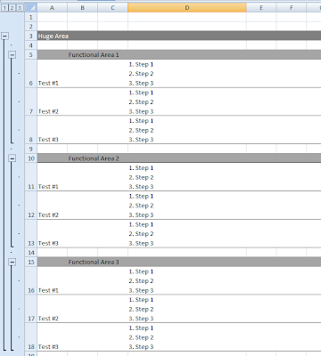
Now in 2020 there is still a lot of test engineers keeping their workouts in MS Excel. That’s easy and fast and all the tests can be easily converted to any other TCMS if your table schema (aka logical schema) is well-designed. One of the best features of Excel which helps a lot of engineers to make their life better is row and column grouping. Using such the feature you may build the visual structure of your test project and collapse and expand certain parts depending on whether you require them. That should look like it is shown on the picture.
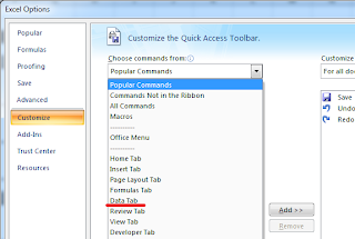
So that’s not the secret how to group the rows. You should switch to data tab, select the rows you’d like to group and click Group button. However the default excel settings cause certain inconvenience. The group headers in such the case are the bottom row of your selected row set. But lets see how to make the header to be at the top. First when you’re starting to design the table, set the cursor to not formatted cell. You have to add new button. Do that using the control as it is shown on the picture. Choose 'More commands…' option.

After you have done it, you should see the dialog of the controls management. Switch the button set to 'Data Tab'
There you should find the control show at the picture below and add it using 'Add>>' button so that it gets to the right-hand list.

So, once it is added, click it

You should see the configuration dialog. Uncheck 'Summary rows below detail' check-box. Click Ok. That’s it. You can now group the rows so that the top one is the group header.
If you still have the questions please send them to me using this form. I will amend the article according to your feedback.